A&S for the 21st century

Sweet, I just discovered that the old classic 1000-page mathematical reference Abramowitz and Stegun has been updated and distributed for the new millennium (well, and century too) in a more modern way.  It's all there free on its own NIST website (the National Institute of Standards and Technology were the ones who published A&S in the first place back in the 1960s).  Here it is right here:

http://dlmf.nist.gov

It was released just two years ago, with both a book version and this online version, which as far as I can tell is a superset of the book.  Here are the three coolest practical aspects of the website version:

1. next to each equation there's a permalink so you can reference a link straight back to the original section of the equation reference
2. and perhaps even better, also next to each equation there's a link to the TeX source for the equation, so you don't even have to rework it all up in TeX again yourself when using it.
3. and even better than that! - ALSO in each section is a list of links to modern software references for finding software libraries & codes to compute the quantities discussed in each section.  (typically in Fortran; note for each code the link puts you at a bibliography entry for a relevant journal paper, but at the right of that ref there's another link that'll get you to the code and other related documents)

NIST Digital Library of Mathematical Functions

(Note the Riemann zeta function used in their cover plot - for these 3D plots you can even interactively go zip around in them via VRML and X3D)

Self-explanatory

Alas this is snipped out of a real geophysics research paper - an important and seminal one at that (Dahlen et al's "banana-donut" paper on ray sensitivity kernels).  So freakin' typical and stereo-typical at the same time...

Tradeoff using central finite differences

Arggg!  (But yay!)  Well my collaborator and I finally figured out why the spectra we were computing were unexpectedly rolling off in the higher wavenumber end.  We were calculating spectra of the derivative of our data series, and were using central finite differences to approximate that derivative.  We'd figured that central differences were more accurate than forward differences and so we were using those (via Matlab's gradient() function), but we realized - ahem, in hindsight - that there's an important tradeoff to be aware of there.  Since the central differences approximate the derivative using the point before and after the present point, it's effectively averaging over three points, and gives you a low-pass filtered version of the derivative.  Forward (and backward) first finite differences do this too but over fewer points (two instead of three) so it's not so big an effect.  The central diffs caused a big enough effect to be a problem in our work, while the forward diffs do not.  Note it depends what aspect of the derivative is most important to you though - phase offset vs frequency rolloff.

In the end we computed the derivative more directly anyway by transforming to the wavenumber domain and multiplying by ik, just to avoid the whole issue.  At any rate, I noticed Terry Bahill (retired from Univ Arizona) has a nice brief paper that sums it up well.  @#$%, can't believe I didn't notice this earlier...

First attempt at using Tableau visualization for estimation results

This is my attempt #1 at using the free Tableau Public visualization software to plot/share results from an example estimation problem, as I explore different approaces to this.  The idea is that there's a LOT of information that comes out of these estimation problems, and it's always hard to figure out how to present it all.  (It's even worse in my continuous inverse problems, as compared to this relatively-simple two-parameter estimation problem... but one thing at a time!)  What intrigues me about Tableau as a possible Tool Of Interest is its purported ability to let a user/viewer (online, say) not merely look at a plot of results, but actually play around with them and explore how they interact.  That would be immensely helpful for trying to understand results that are commonly computed in my field.

This example problem here is an MCMC (Markov-Chain Monte Carlo) approach to solving Problem 7.1 in Albert Tarantola's Inverse Problem Theory book (amazingly available free online in addition to bookstores), a simple version of finding a seismic source based on arrival times at receiver stations.  It's the same problem as is solved by linearization techniques in my Lab#4  (scroll to bottom) for the UW Inverse Theory class that I worked up with Professor Ken Creager.  I have a whole webpage coming at some point in near future explaining how this problem example is done with both techniques and providing Matlab/Octave code for it.  For now I realize this may be a pile of jargon if you're not yet familiar with the techniques or physics of the problem, as I don't actually describe them here (gotta go read the lab page or the book above!).  At any rate, for those at least a little familiar with the problem and/or method, the "map-view" portion of the problem's objective function looks like the following.

The triangles in upper left corner are receivers that recorded (simulated) earthquake or acoustic transmissions from a source whose location we wish to estimate from the varying arrival times on those receivers.  However, since the receivers are so close together compared to the distance to the source, the azimuth angle of the source isn't well resolved even if the radial distance is - you get this arc-shaped uncertainty region reflecting this fact.  The MCMC sampling approach can accurately give you this arc (with colors depicting the probability of the source's location along the arc, i.e. white is really low probability); that's unlike the "straight" error ellipse that the linearization technique in our Lab#4 can give - this is the difference between a fully nonlinear vs linear approximation to the solution uncertainties in this problem.  

So that's a great advantage of MCMC, but the only thing is, there's a big catch - this next plot here gives some feel for the number of computational steps that the MCMC approach required (in color) compared to the handful required by the linearization approach in Lab#4 (in black and white).  It was something like a million steps compared to five.  So there's a very big tradeoff indeed!  Notice they start from the same initial-estimate point (I think that's 15,15 or so) and they result in approximately the same highest-probability location for the source (white-circle endpoint on top of reddest region), but the difference in the uncertainties for those two solutions (arc vs ellipse) is the real difference between the two techniques in this problem.

Anyways, so my interest here was playing with how the various aspects of the results could be presented and explored with new tools... so I thought I'd play with Tableau a little bit.  The embedded result is at the bottom of this post (expect something dull and limited - this is my first try!).  There are a lot of basics I haven't figured out how to do yet here - even super basic stuff like adding on the original receiver locations superimposed onto the north/east geographic plot, or connecting the orange points on that plot with lines so we can see the path of the random walk used in the MCMC computation - so far I think my Matlab plots above are way more informative.  But hopefully such basics are easy and doable in Tableau and presumably I simply didn't manage to figure them out in my brief playing around here.  My data file that I'm basing it out of is a single six-column ASCII file (or 7 if you include the one for record-number as I couldn't find an automatic field for that yet in Tableau) that was produced by my MCMC computation that was killed halfway through (Tableau Public has a record-limit so that'd be an issue anyway), so you'll note the chopped-off nature of the orange plot below.  Columns included sample #, posterior probability, prior probability, acceptance rate, param#1 (north), param#2 (east), and there's a number of useful ways to look at several of these quantities at a time.  Again something I particularly like is the idea that the user can interact with the plots.  In the embedded plots below, it seems you can double click to zoom in on data regions (haven't figured out how to zoom back out yet!), and get a pop-up box that lists the other data quantities associated with the plotted point (I think there's a way to get all six fields listed there).  Among other things I'd like to figure out how to click a point in one plot and show its counterpart in the other plots.

Lastly, a quick troubleshooting note on my use of Tableau Public itself - I ran it in a virtual machine with old Windows XP installed in it (actually tried both VirtualBox and VMware), and on my first tries I could run the whole program until trying to "Save to Web" (their server), when I'd get this error message:

I spent a bit verifying that I had internet connectivity and correct ports open and Tableau Public account correctly set up and so on, to no avail.  Turns out that to do the upload to their server, Tableau apparently relies on built-in functionality from the more recent releases of Microsoft Internet Explorer than I had installed - once I ran Windows Update and brought the IEv6 I had up to IEv8, it all worked fine.  (Would be nice if the error messages were more informative.)

Alright, well, I look forward to the next iteration of my Tableau attempts for estimation problems like this in the near future.  I really like the idea of this tool... even if I haven't yet figured out how to best suit it to my own needs.

Powered by Tableau

Installing G77 on Ubuntu 10.04 & 11.10

Alas some of the wave propagation codes I use on my v10.04 and v11.10 Ubuntu Linux systems require the outdated g77 compiler.

However, g77 is no longer being maintained and was last made to support GCC 3.4.  More recent Ubuntu versions use GCC 4.X and so dropped g77 from their default package manager lists.  Took a little bit to figure out how to get the relevant stuff installed and working on these computers, as I still needed the GCC 4.X for other content on the machines.  Here's what I did:

The overall summary is, to get g77 and its libraries you have to temporarily modify an apt-get repository list file, install g77 (which automatically also installs its GCC 3.4 dependencies which won't interfere with your gcc 4.x), and then set the repository file back to its original state.  Also, there's an additional little fix to install g77 in Ubuntu 11.10 that wasn't in Ubuntu 10.04 (I haven't tried the versions of Ubuntu in between): a few libs moved location, so you simply use an environment variable to tell g77 where they are.  Steps detailed below:

sudo vi /etc/apt/sources.list, then append the following lines to end of file:

## temporarily adding these to install G77 which is no longer supported:
deb http://hu.archive.ubuntu.com/ubuntu/ hardy universe
deb-src http://hu.archive.ubuntu.com/ubuntu/ hardy universe
deb http://hu.archive.ubuntu.com/ubuntu/ hardy-updates universe
deb-src http://hu.archive.ubuntu.com/ubuntu/ hardy-updates universe

sudo aptitude update

sudo aptitude install g77 blcr-dkms: blcr-util: dkms: fakeroot: libcr0: libibverbs-dev: openmpi-common:
(Those entries with colons afterward prevent those packages from being removed to match the outdated setup, which we don't wish to do)

sudo vi /etc/apt/sources.list again and comment out those above lines at end of file.

sudo aptitude update

If you're running Ubuntu 11.10 (but this is not needed for 10.04; I don't know about versions in between, the error is about finding libs crt1.o, crti.o and lgcc_s):
Before running make (or g77 in general) you'll need to enter the following line in your shell (note this is bash style here, mod as needed for other shells):

export LIBRARY_PATH=/usr/lib/x86_64-linux-gnu:/usr/lib/gcc/x86_64-linux-gnu/4.6

(Note that is not the more common variable LD_LIBRARY_PATH...)

If you plan to do a lot of g77 compiles you might wish to add that LIBRARY_PATH line to your ~/.bashrc file, but for just one or two compiles I personally choose not to do so.

Note that executables made with this g77 may rely by default on shared object libraries of g77/gcc 3.4, so if you copy your executable over to other modern Linux systems (say another 10.04 or 11.10 box -- e.g. I use mine in a cluster), you may get a runtime error about shared object files.  The solution is to install g77 on that other system as well by the same instructions above, so that the shared object files exist.  It goes pretty quickly after the first time.

The GNU "Screen" command

If you frequently program and run computations on a remote Linux/Unix computer, maybe you're familiar with this scenario that I often find myself in:  Working in six different terminal logins to the remote computer from the office desktop computer, cranking up long-running computations that are still not finished and are outputting important information (calculation status or results), but it's time to catch the bus home.  On the bus I realized I started one of the computations with a wrong parameter, so I login from my iPhone to fix and restart it, but I have to setup the whole environment again (cd, restart octave, load data or scripts etc) in this new login.  Then I get home and later after the wife and kids are in bed I'm logging in again... and have to set up the whole environment again with my new set of six logins.  And the following morning when I come back to the office the same thing happens.

Enter the long-existing and very simple, but totally indispensable GNU screen command.  It's maybe a bit similar to emacs (if you're familiar with that all-but-kitchen-sink text editor), in terms of letting you set up different tiled windows and buffers and shells that you can rearrange and swap between; maybe a bit more of a vi style to it than an emacs style.  But the real key is its ability to let you completely detach the entire thing from one terminal and reattach it intact from a different terminal login.  As far as I know, that's something that emacs can't do!  So imagine I've got an emacs-like setup with six (or whatever) window buffers in some kind of container, and when I go login on the bus from my iPhone I call up that container to my iPhone screen, and when I login from my computer at home I pull the container to that login terminal, and then the next morning pull it back up on my office computer.  All the window buffers are still intact the whole time so I don't have to worry about elaborate background-writing-stdout-to-status-files if I don't want to bother.

There are man pages and instruction pages all over the web for it, so I won't bother with that here, but here's one of the instruction webpages that I found handy when getting started.

Something that isn't so obvious when getting started is how to set up your status line at the bottom of the window, which shows e.g. which window buffers you have, which currently holds the cursor, and whatever else you put in there like time or system load.  I'd start with putting the following cryptic lines in your ~/.screenrc file (which I use for my own status line) and start playing from there, probably also referencing a webpage such as this one.


caption splitonly "%{= ky}%H-%n (%t)"
hardstatus on
hardstatus alwayslastline
hardstatus string "%{.kr}%-w%{.ky}%n-%t%{.kr}%+w %75=%{.kg}%H load: %l"  # sysload but no time/date
#hardstatus string "%{.kr}%-w%{.ky}%n-%t%{.kr}%+w %35=%{.kg}%H load: %l %{.kc}%=%c  %{.km}%D %d %M %Y"  # sysload + time/date

Here's an example of what a screen session might look like on my computer - six logins but only two presently showing:

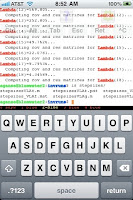
And here's what it looks like on my iPhone in the TouchTerm app:

I tell you, this command totally saves my sanity during weeks when I have to focus on cranking out calculations on our computer cluster.

Just lastly, a handy thing to be aware of regarding GNU screen is that for some reason a number of distros of screen don't have the vertical window split (as compared to the horizontal split seen above) compiled in.  It's a handy feature, and here's a webpage that explains how to patch screen's source code and recompile to get that feature.

Octave plots in ASCII - just like the old days!

Well whattya know.  Another Octave feature here; I stumbled across this when finding a solution to the following original problem.  I was looping to make a large number of plots that I was printing to pdf files, and since it was taking a while and the new plots kept getting in my way on the screen, I turned off the screen plots via:

h=figure;
set(h,'visible','off');
plot...

Problem was, while that stopped the plots from showing on the screen, still every time a new plot figure was called the cursor focus would go back to the X11 app (I'm on OSX) which made it awfully frustrating to work in another terminal window.  (This doesn't happen in Matlab by the way; in Matlab the set(h,'visible','off') appears to be enough.)  After much searching and experimentation I finally discovered that I could preface the above with a line to change the graphics terminal type in Octave to cut X11 out of the loop, like this:

putenv('GNUTERM','dumb');

That form works in Octave 3.4.0; the earlier form of "set terminal dumb" doesn't seem to work anymore.  Anyway, that solved my trouble of the reverting cursor focus and made me happy.  But then I found what else that dumb-terminal setting is good for -- making good old-fashioned ASCII plots!  Remember those?  I suppose you need to be of a certain age to really appreciate this.  Here's the idea by way of an example:


octave-3.4.0:15:44:07> putenv('LINES','30');
octave-3.4.0:15:48:54> putenv('COLUMNS','70');
octave-3.4.0:15:48:56> putenv('GNUTERM','dumb');
octave-3.4.0:15:48:59> plot(r_TCTD,c_TCTD([1,3,5],:)); \
> xlabel('range (km)'); title('soundspeeds (m/s) in towed seacable sensors')
+--------------------------------------------------------------------+
|              soundspeeds (m/s) in towed seacable sensors           |
|                                                                    |
|1540 ++--------+---------+---------+---------+---------+--------++  |
|     +         +         +         +         +         +         +  |
|     |                                                           |  |
|1538 ++++++++                                                   ++  |
|     |     +++++++++++                                    +      |  |
|     |               ++++      +++++++                ++++++     |  |
|1536 ++                 ++++++++++  +++++++++++++++++++ +       ++  |
|     |                                              ++           |  |
|     |  +                                                        |  |
|1534 ++++++++++    +                                            ++  |
|     |   +  ++++++++++                                           |  |
|     |              ++++++++      +++++++ ++++  +                |  |
|1532 ++                  ++++++++++    ++++ ++++++++++++ +++    ++  |
|     |                      +++++                    +++++       |  |
|     |  +  +                                            +        |  |
|1530 ++++++++++ +++++                                           ++  |
|     |      + +++   +                ++                          |  |
|     |              ++++          +++++++ ++++++                 |  |
|1528 ++              + +++++++++++++   ++++ ++++++++            ++  |
|     |                   + ++ ++                  +++++ ++++     |  |
|     +         +         +         +         +        +++ ++     +  |
|1526 ++--------+---------+---------+---------+---------+--------++  |
|    440       445       450       455       460       465       470 |
|                              range (km)                            |
+--------------------------------------------------------------------+


And there you have it -- plot your stuff to the ASCII terminal instead of some boring old publication quality PS or PDF file!  Now, WHY would you ever bother to do this?  Ok, honestly I can't really think of a reason, but it's the way we used to check over results on-screen before printing out to the printer, you know, kindof a few years ago.  Just think of it as "retro"...

Hey, it was good for 10 minutes of mindless diversion in any case!  And I do have the excuse that finding this dumb-terminal setting really saved the day for turning off the on-screen plots/focus issue.  Just lastly, note I did find that this ASCII plotting didn't work in Octave v3.2.3, but the dumb terminal is still available in that version by the same command, and at least still took care of the screen-focus issue.

LaTeX labels in Matlab and Octave

Very happy to've finally discovered the LaTeX interpreter option in Matlab labels this evening.  Previously I'd been so frustrated when wanting to use something mathy like a partial derivative expression to label a plot axis, because while I can specify a few LaTeX-like things in there like partials and sub/superscripts:


xlabel('\partial{P_k}(t_i)/\partial{S}_{p}(z_j)');

it comes out looking kinda lame like this:

I mean, it's not totally unusable (been using it that way for years in fact!), but it's all scrunched up against the axis numbers and the subscript spacing is screwy and the relative sizes of the partials and variables is lousy; just not very professional looking.  Octave (awesome free GNU clone of Matlab) which I often use does better with that same unmodified xlabel line:

but it's still not ideal.

Turns out in Matlab you can modify that label statement and call its built-in LaTeX interpreter like so:


xlabel( '$\partial{P_k}(t_i)/\partial{S}_\mathrm{p}(z_j)$', 'Interpreter', 'latex' );

The flanking $'s denote math-mode to the LaTeX interpreter, and note added in the \mathrm{} to improve that p subscript, which you couldn't use above since it wasn't really LaTeX handling the above.  Anyway, with LaTeX now it looks like this:

Much better!  I did find a little remaining funniness - that result there was after having first specified a 14pt font size on the axes text via:

set(0,'DefaultAxesFontSize',14); 

But using the LaTeX interpreter for xlabel with the original default fontsize had some subscript spacing issues (k subscript touching paren and wide space before the p subscript):

As far as an equivalent in Octave, according to the latest in the user manual under Section 15.2.8, "Use of the interpreter Property", that 'latex' interpreter option isn't implemented yet (although the hook is there).  The 'tex' interpreter option that's mentioned in that section is just the bit that was shown at the top of this post, which Octave does do a little better than Matlab but it's pretty limited.  There are a few webpages I've seen (e.g. here and here) about how to output an EPS plot file from Octave and then pass it through latex with a specially written .tex file to use the full interpreter that way.  But that too much effort for me.  Meanwhile I'm just happy I've figured out the LaTeX use in Matlab at least.

Subplot spacing in Octave 3.2.3

Figured out how to fix the terrible spacing troubles with subplots in Octave 3.2.3.  They were coming out overlapped and squished on top of each other, clearly a bug, but on machines that I didn't have Matlab on I'd just have to manually fix it up each time by adding in a bunch of set(h,'position'... statements in the scripts, which would then need to be manually fudged and updated if anything else changed.  Bleah.


This was fixed for Octave 3.4.0 but that version is not out in easily updatable binaries for all OS distributions yet and I was stuck with Octave 3.2.3.  But I finally found it's an easy fix - no recompiling or anything, just a one-line tweak in an m-file.  (You'll notice this file is on my Mac but it's a problem on all platforms, and you can find this same file in its respective folder on other OS's too...)

In the file 
/Applications/Octave.app/Contents/Resources/share/octave/3.2.3/m/plot/__go_draw_axes__.m, 
replace line 50 (after making a backup copy of the file):

 ## pos = pos - implicit_margin([1, 2, 1, 2]).*[1, 1, -0.5, -0.5];

with:

 pos(1:2) = pos(1:2) - implicit_margin .* [0.75, 0.5];

And that's it.  Note this is based on Ben Abbot's fix for Octave v3.4.0 at  https://savannah.gnu.org/bugs/index.php?29656

Hm, however the problem seems to remain for image and imagesc though, those must be in a separate call...

Tarantola's new physics book

This is kindof an interesting idea (just recently read the intro to this book):  You know how vectors are defined independently of any coordinate system -- they're specific points in space regardless of how you name those points, and e.g. their sum and so on is the same regardless of coord system.  For those who've done a little higher level physics you've seen this is true for tensors in general.  Well, so Albert Tarantola's point in his new textbook Elements for Physics (having only read the intro, mind you) is that our laws of physics are all derived or empirically found in a particular coordinate system, but the quantities they describe needn't be -- for example a scale of temperature could be quantified via the temperature value, the inverse temperature, log temperature, etc., but any given value of one of these quantities is still talking about a particular hotness/coldness.  And his thought is that rather than have one equation that relates temperature to say heat flux, another equation to relate the inverse temp, and another for log temp (even though these particular examples might be simply related), he would go derive the equivalent of those which instead relates the invariant quantities and try to learn something more fundamental about their relationship in the process.  At the end one can always take the invariant quantity and express it in a given coord system.  Ideally that would produce the original historical physics law, and in his examples generally did but at least once apparently didn't (heat flux vs temp, Fourier's Law), which is surprising, not sure came of that.  Anyway, as with his wonderful inverse theory textbook he offers this one in a PDF file free online, with the understanding that if you can afford it and use it then please buy it...