Installing G77 on Ubuntu 10.04 & 11.10

Alas some of the wave propagation codes I use on my v10.04 and v11.10 Ubuntu Linux systems require the outdated g77 compiler.

However, g77 is no longer being maintained and was last made to support GCC 3.4.  More recent Ubuntu versions use GCC 4.X and so dropped g77 from their default package manager lists.  Took a little bit to figure out how to get the relevant stuff installed and working on these computers, as I still needed the GCC 4.X for other content on the machines.  Here's what I did:

The overall summary is, to get g77 and its libraries you have to temporarily modify an apt-get repository list file, install g77 (which automatically also installs its GCC 3.4 dependencies which won't interfere with your gcc 4.x), and then set the repository file back to its original state.  Also, there's an additional little fix to install g77 in Ubuntu 11.10 that wasn't in Ubuntu 10.04 (I haven't tried the versions of Ubuntu in between): a few libs moved location, so you simply use an environment variable to tell g77 where they are.  Steps detailed below:

sudo vi /etc/apt/sources.list, then append the following lines to end of file:

## temporarily adding these to install G77 which is no longer supported:
deb http://hu.archive.ubuntu.com/ubuntu/ hardy universe
deb-src http://hu.archive.ubuntu.com/ubuntu/ hardy universe
deb http://hu.archive.ubuntu.com/ubuntu/ hardy-updates universe
deb-src http://hu.archive.ubuntu.com/ubuntu/ hardy-updates universe

sudo aptitude update

sudo aptitude install g77 blcr-dkms: blcr-util: dkms: fakeroot: libcr0: libibverbs-dev: openmpi-common:
(Those entries with colons afterward prevent those packages from being removed to match the outdated setup, which we don't wish to do)

sudo vi /etc/apt/sources.list again and comment out those above lines at end of file.

sudo aptitude update

If you're running Ubuntu 11.10 (but this is not needed for 10.04; I don't know about versions in between, the error is about finding libs crt1.o, crti.o and lgcc_s):
Before running make (or g77 in general) you'll need to enter the following line in your shell (note this is bash style here, mod as needed for other shells):

export LIBRARY_PATH=/usr/lib/x86_64-linux-gnu:/usr/lib/gcc/x86_64-linux-gnu/4.6

(Note that is not the more common variable LD_LIBRARY_PATH...)

If you plan to do a lot of g77 compiles you might wish to add that LIBRARY_PATH line to your ~/.bashrc file, but for just one or two compiles I personally choose not to do so.

Note that executables made with this g77 may rely by default on shared object libraries of g77/gcc 3.4, so if you copy your executable over to other modern Linux systems (say another 10.04 or 11.10 box -- e.g. I use mine in a cluster), you may get a runtime error about shared object files.  The solution is to install g77 on that other system as well by the same instructions above, so that the shared object files exist.  It goes pretty quickly after the first time.

The GNU "Screen" command

If you frequently program and run computations on a remote Linux/Unix computer, maybe you're familiar with this scenario that I often find myself in:  Working in six different terminal logins to the remote computer from the office desktop computer, cranking up long-running computations that are still not finished and are outputting important information (calculation status or results), but it's time to catch the bus home.  On the bus I realized I started one of the computations with a wrong parameter, so I login from my iPhone to fix and restart it, but I have to setup the whole environment again (cd, restart octave, load data or scripts etc) in this new login.  Then I get home and later after the wife and kids are in bed I'm logging in again... and have to set up the whole environment again with my new set of six logins.  And the following morning when I come back to the office the same thing happens.

Enter the long-existing and very simple, but totally indispensable GNU screen command.  It's maybe a bit similar to emacs (if you're familiar with that all-but-kitchen-sink text editor), in terms of letting you set up different tiled windows and buffers and shells that you can rearrange and swap between; maybe a bit more of a vi style to it than an emacs style.  But the real key is its ability to let you completely detach the entire thing from one terminal and reattach it intact from a different terminal login.  As far as I know, that's something that emacs can't do!  So imagine I've got an emacs-like setup with six (or whatever) window buffers in some kind of container, and when I go login on the bus from my iPhone I call up that container to my iPhone screen, and when I login from my computer at home I pull the container to that login terminal, and then the next morning pull it back up on my office computer.  All the window buffers are still intact the whole time so I don't have to worry about elaborate background-writing-stdout-to-status-files if I don't want to bother.

There are man pages and instruction pages all over the web for it, so I won't bother with that here, but here's one of the instruction webpages that I found handy when getting started.

Something that isn't so obvious when getting started is how to set up your status line at the bottom of the window, which shows e.g. which window buffers you have, which currently holds the cursor, and whatever else you put in there like time or system load.  I'd start with putting the following cryptic lines in your ~/.screenrc file (which I use for my own status line) and start playing from there, probably also referencing a webpage such as this one.


caption splitonly "%{= ky}%H-%n (%t)"
hardstatus on
hardstatus alwayslastline
hardstatus string "%{.kr}%-w%{.ky}%n-%t%{.kr}%+w %75=%{.kg}%H load: %l"  # sysload but no time/date
#hardstatus string "%{.kr}%-w%{.ky}%n-%t%{.kr}%+w %35=%{.kg}%H load: %l %{.kc}%=%c  %{.km}%D %d %M %Y"  # sysload + time/date

Here's an example of what a screen session might look like on my computer - six logins but only two presently showing:

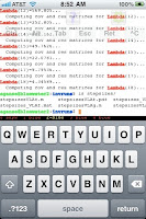
And here's what it looks like on my iPhone in the TouchTerm app:

I tell you, this command totally saves my sanity during weeks when I have to focus on cranking out calculations on our computer cluster.

Just lastly, a handy thing to be aware of regarding GNU screen is that for some reason a number of distros of screen don't have the vertical window split (as compared to the horizontal split seen above) compiled in.  It's a handy feature, and here's a webpage that explains how to patch screen's source code and recompile to get that feature.

Octave plots in ASCII - just like the old days!

Well whattya know.  Another Octave feature here; I stumbled across this when finding a solution to the following original problem.  I was looping to make a large number of plots that I was printing to pdf files, and since it was taking a while and the new plots kept getting in my way on the screen, I turned off the screen plots via:

h=figure;
set(h,'visible','off');
plot...

Problem was, while that stopped the plots from showing on the screen, still every time a new plot figure was called the cursor focus would go back to the X11 app (I'm on OSX) which made it awfully frustrating to work in another terminal window.  (This doesn't happen in Matlab by the way; in Matlab the set(h,'visible','off') appears to be enough.)  After much searching and experimentation I finally discovered that I could preface the above with a line to change the graphics terminal type in Octave to cut X11 out of the loop, like this:

putenv('GNUTERM','dumb');

That form works in Octave 3.4.0; the earlier form of "set terminal dumb" doesn't seem to work anymore.  Anyway, that solved my trouble of the reverting cursor focus and made me happy.  But then I found what else that dumb-terminal setting is good for -- making good old-fashioned ASCII plots!  Remember those?  I suppose you need to be of a certain age to really appreciate this.  Here's the idea by way of an example:


octave-3.4.0:15:44:07> putenv('LINES','30');
octave-3.4.0:15:48:54> putenv('COLUMNS','70');
octave-3.4.0:15:48:56> putenv('GNUTERM','dumb');
octave-3.4.0:15:48:59> plot(r_TCTD,c_TCTD([1,3,5],:)); \
> xlabel('range (km)'); title('soundspeeds (m/s) in towed seacable sensors')
+--------------------------------------------------------------------+
|              soundspeeds (m/s) in towed seacable sensors           |
|                                                                    |
|1540 ++--------+---------+---------+---------+---------+--------++  |
|     +         +         +         +         +         +         +  |
|     |                                                           |  |
|1538 ++++++++                                                   ++  |
|     |     +++++++++++                                    +      |  |
|     |               ++++      +++++++                ++++++     |  |
|1536 ++                 ++++++++++  +++++++++++++++++++ +       ++  |
|     |                                              ++           |  |
|     |  +                                                        |  |
|1534 ++++++++++    +                                            ++  |
|     |   +  ++++++++++                                           |  |
|     |              ++++++++      +++++++ ++++  +                |  |
|1532 ++                  ++++++++++    ++++ ++++++++++++ +++    ++  |
|     |                      +++++                    +++++       |  |
|     |  +  +                                            +        |  |
|1530 ++++++++++ +++++                                           ++  |
|     |      + +++   +                ++                          |  |
|     |              ++++          +++++++ ++++++                 |  |
|1528 ++              + +++++++++++++   ++++ ++++++++            ++  |
|     |                   + ++ ++                  +++++ ++++     |  |
|     +         +         +         +         +        +++ ++     +  |
|1526 ++--------+---------+---------+---------+---------+--------++  |
|    440       445       450       455       460       465       470 |
|                              range (km)                            |
+--------------------------------------------------------------------+


And there you have it -- plot your stuff to the ASCII terminal instead of some boring old publication quality PS or PDF file!  Now, WHY would you ever bother to do this?  Ok, honestly I can't really think of a reason, but it's the way we used to check over results on-screen before printing out to the printer, you know, kindof a few years ago.  Just think of it as "retro"...

Hey, it was good for 10 minutes of mindless diversion in any case!  And I do have the excuse that finding this dumb-terminal setting really saved the day for turning off the on-screen plots/focus issue.  Just lastly, note I did find that this ASCII plotting didn't work in Octave v3.2.3, but the dumb terminal is still available in that version by the same command, and at least still took care of the screen-focus issue.

LaTeX labels in Matlab and Octave

Very happy to've finally discovered the LaTeX interpreter option in Matlab labels this evening.  Previously I'd been so frustrated when wanting to use something mathy like a partial derivative expression to label a plot axis, because while I can specify a few LaTeX-like things in there like partials and sub/superscripts:


xlabel('\partial{P_k}(t_i)/\partial{S}_{p}(z_j)');

it comes out looking kinda lame like this:

I mean, it's not totally unusable (been using it that way for years in fact!), but it's all scrunched up against the axis numbers and the subscript spacing is screwy and the relative sizes of the partials and variables is lousy; just not very professional looking.  Octave (awesome free GNU clone of Matlab) which I often use does better with that same unmodified xlabel line:

but it's still not ideal.

Turns out in Matlab you can modify that label statement and call its built-in LaTeX interpreter like so:


xlabel( '$\partial{P_k}(t_i)/\partial{S}_\mathrm{p}(z_j)$', 'Interpreter', 'latex' );

The flanking $'s denote math-mode to the LaTeX interpreter, and note added in the \mathrm{} to improve that p subscript, which you couldn't use above since it wasn't really LaTeX handling the above.  Anyway, with LaTeX now it looks like this:

Much better!  I did find a little remaining funniness - that result there was after having first specified a 14pt font size on the axes text via:

set(0,'DefaultAxesFontSize',14); 

But using the LaTeX interpreter for xlabel with the original default fontsize had some subscript spacing issues (k subscript touching paren and wide space before the p subscript):

As far as an equivalent in Octave, according to the latest in the user manual under Section 15.2.8, "Use of the interpreter Property", that 'latex' interpreter option isn't implemented yet (although the hook is there).  The 'tex' interpreter option that's mentioned in that section is just the bit that was shown at the top of this post, which Octave does do a little better than Matlab but it's pretty limited.  There are a few webpages I've seen (e.g. here and here) about how to output an EPS plot file from Octave and then pass it through latex with a specially written .tex file to use the full interpreter that way.  But that too much effort for me.  Meanwhile I'm just happy I've figured out the LaTeX use in Matlab at least.

Subplot spacing in Octave 3.2.3

Figured out how to fix the terrible spacing troubles with subplots in Octave 3.2.3.  They were coming out overlapped and squished on top of each other, clearly a bug, but on machines that I didn't have Matlab on I'd just have to manually fix it up each time by adding in a bunch of set(h,'position'... statements in the scripts, which would then need to be manually fudged and updated if anything else changed.  Bleah.


This was fixed for Octave 3.4.0 but that version is not out in easily updatable binaries for all OS distributions yet and I was stuck with Octave 3.2.3.  But I finally found it's an easy fix - no recompiling or anything, just a one-line tweak in an m-file.  (You'll notice this file is on my Mac but it's a problem on all platforms, and you can find this same file in its respective folder on other OS's too...)

In the file 
/Applications/Octave.app/Contents/Resources/share/octave/3.2.3/m/plot/__go_draw_axes__.m, 
replace line 50 (after making a backup copy of the file):

 ## pos = pos - implicit_margin([1, 2, 1, 2]).*[1, 1, -0.5, -0.5];

with:

 pos(1:2) = pos(1:2) - implicit_margin .* [0.75, 0.5];

And that's it.  Note this is based on Ben Abbot's fix for Octave v3.4.0 at  https://savannah.gnu.org/bugs/index.php?29656

Hm, however the problem seems to remain for image and imagesc though, those must be in a separate call...

Tarantola's new physics book

This is kindof an interesting idea (just recently read the intro to this book):  You know how vectors are defined independently of any coordinate system -- they're specific points in space regardless of how you name those points, and e.g. their sum and so on is the same regardless of coord system.  For those who've done a little higher level physics you've seen this is true for tensors in general.  Well, so Albert Tarantola's point in his new textbook Elements for Physics (having only read the intro, mind you) is that our laws of physics are all derived or empirically found in a particular coordinate system, but the quantities they describe needn't be -- for example a scale of temperature could be quantified via the temperature value, the inverse temperature, log temperature, etc., but any given value of one of these quantities is still talking about a particular hotness/coldness.  And his thought is that rather than have one equation that relates temperature to say heat flux, another equation to relate the inverse temp, and another for log temp (even though these particular examples might be simply related), he would go derive the equivalent of those which instead relates the invariant quantities and try to learn something more fundamental about their relationship in the process.  At the end one can always take the invariant quantity and express it in a given coord system.  Ideally that would produce the original historical physics law, and in his examples generally did but at least once apparently didn't (heat flux vs temp, Fourier's Law), which is surprising, not sure came of that.  Anyway, as with his wonderful inverse theory textbook he offers this one in a PDF file free online, with the understanding that if you can afford it and use it then please buy it...